---
title: "Cookbook"
author: "Jeremy Wildfire"
date: "`r Sys.Date()`"
output: rmarkdown::html_vignette
vignette: >
%\VignetteIndexEntry{Cookbook}
%\VignetteEngine{knitr::rmarkdown}
%\VignetteEncoding{UTF-8}
---
# Cookbook Vignette
This vignette contains a series of examples showing how to initialize the safetyGraphics Shiny app in different scenarios.
# Overview
Most of the customization shown here is done by changing 4 key parameters in the `safetyGraphicsApp()` function:
- `domainData` – Domain-level Study Data
- `mapping` – List identifying the key columns/fields in your data
- `charts` – Define the charts used in the app.
- `meta` – Metadata table with info about required columns and fields
`domainData` and `mapping` generally change for every study, while `charts` and `meta` can generally be re-used across many studies.
The examples here are generally provided with minimal explanation. For a more detailed discussion of the logic behind these examples see the [Chart Configuration Vignette](ChartConfiguration.html) or our [2021 R/Pharma Workshop](https://github.com/SafetyGraphics/RPharma2021-Workshop)
# Setup and installation
safetyGraphics requires R v4 or higher. These examples have been tested using RStudio v1.4, but should work on other platforms with proper configuration.
You can install `{safetyGraphics}` from CRAN like any other R package:
```
install.packages("safetyGraphics")
library("safetyGraphics")
```
Or to use the most recent development version from GitHub, call:
```
devtools::install_github("safetyGraphics/safetyCharts", ref="dev")
library(safetyCharts)
devtools::install_github("safetyGraphics/safetyGraphics", ref="dev")
library(safetyGraphics)
safetyGraphics::safetyGraphicsApp()
```
## Example 1 - Default App
To run the app with no customizations using sample AdAM data from the {safetyData} package, install the package and run:
```
safetyGraphics::safetyGraphicsApp()
```
# Loading Custom Data
The next several examples focus on study-specific customizations for loading and mapping data.
## Example 2 - SDTM Data
The data passed in to the safetyGraphics app can be customized using the `domainData` parameter in `safetyGraphicsApp()`. For example, to run the app with SDTM data saved in `{safetyData}`, call:
```
sdtm <- list(
dm=safetyData::sdtm_dm,
aes=safetyData::sdtm_ae,
labs=safetyData::sdtm_lb
)
safetyGraphics::safetyGraphicsApp(domainData=sdtm)
```
## Example 3 - Single Data Domain
Running the app for a single data domain, is similar:
```
justLabs <- list(labs=safetyData::adam_adlbc)
safetyGraphics::safetyGraphicsApp(domainData=justLabs)
```
Note that charts with missing data are automatically dropped and the filtering tab is not present since it requires demographics data by default.
## Example 4 - Loading other data formats
Users can also import data from a wide-variety of data formats using standard R workflows and then initialize the app. The example below initializes the app using lab data saved as a sas transport file (.xpt)
```
xptLabs <- haven::read_xpt('https://github.com/phuse-org/phuse-scripts/blob/master/data/adam/cdiscpilot01/adlbc.xpt?raw=true')
safetyGraphics::safetyGraphicsApp(domainData=list(labs=xptLabs))
```
## Example 5 - Non-standard data
Next, let's initialize the the app with non-standard data. {safetyGraphics} automatically detects AdAM and SDTM data when possible, but for non-standard data, the user must provide a data mapping. This can be done in the app using the data/mapping tab, or can be done when the app is initialized by passing a `mapping` list to `safetyGraphicsApp()`. For example:
```
notAdAM <- list(labs=safetyData::adam_adlbc %>% rename(id = USUBJID))
idMapping<- list(labs=list(id_col="id"))
safetyGraphicsApp(domainData=notAdAM, mapping=idMapping)
```
## Example 6 - Non-standard data #2
For a more realistic example, consider [this labs data set (csv)](https://raw.githubusercontent.com/SafetyGraphics/SafetyGraphics.github.io/master/pilot/SampleData_NoStandard.csv). The data can be loaded in to safetyGraphics with the code below, but several items in the mapping page need to be filled in:
```
labs <- read.csv("https://raw.githubusercontent.com/SafetyGraphics/SafetyGraphics.github.io/master/pilot/SampleData_NoStandard.csv")
safetyGraphics::safetyGraphicsApp(domainData=list(labs=labs))
```
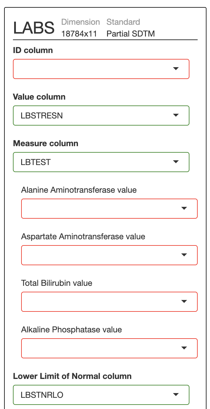 Fortunately there is no need to re-enter this mapping information in every time you re-start the app. After filling in these values once, you can export code to restart the app *with the specified settings pre-populated*. First, click on the setting icon in the header and then on "code" to see this page:
 The YAML code provided here captures the updates you've made on the mapping page. To re-start the app with those settings, just save these YAML code in a new file called `customSettings.yaml` in your working directory, and then call:
```
labs <- read.csv("https://raw.githubusercontent.com/SafetyGraphics/SafetyGraphics.github.io/master/pilot/SampleData_NoStandard.csv")
customMapping <- read_yaml("customSettings.yaml")
safetyGraphics::safetyGraphicsApp(
domainData=list(labs=labs),
mapping=customMapping
)
```
Note, that for more complex customizations, the setting page also provides a `.zip` file with a fully re-usable version of the app.
# Custom Charts
The remaining examples focus on creating charts that are reusable across many studies. For extensive details on adding and customizing different types of charts, see this [vignette](ChartConfiguration.html).
## Example 7 - Drop Unwanted Charts
Users can also generate a list of charts and then drop charts that they don't want to include. For example, if you wanted to drop charts with `type` of "htmlwidgets" you could run this code.
```
library(purrr)
charts <- makeChartConfig() #gets charts from safetyCharts pacakge by default
notWidgets <- charts %>% purrr::keep(~.x$type != "htmlwidget")
safetyGraphicsApp(charts=notWidgets)
```
## Example 8 - Edit Default Charts
Users can also make modifications to the default charts by editing the list of charts directly.
```
charts <- makeChartConfig() #gets charts from safetyCharts pacakge by default
charts$aeTimelines$label <- "An AMAZING timeline"
safetyGraphicsApp(charts=charts)
```
## Example 9 - Add Hello World Custom Chart
This example creates a simple "hello world" chart that is not linked to the data or mapping loaded in the app.
```
helloWorld <- function(data, settings){
plot(-1:1, -1:1)
text(runif(20, -1,1),runif(20, -1,1),"Hello World")
}
# Chart Configuration
helloworld_chart<-list(
env="safetyGraphics",
name="HelloWorld",
label="Hello World!",
type="plot",
domain="aes",
workflow=list(
main="helloWorld"
)
)
safetyGraphicsApp(charts=list(helloworld_chart))
```
## Example 10 - Add a custom chart using data and settings
The code below adds a new simple chart showing participants' age distribution by sex.
```
ageDist <- function(data, settings){
p<-ggplot(data = data, aes(x=.data[[settings$age_col]])) +
geom_histogram() +
facet_wrap(settings$sex_col)
return(p)
}
ageDist_chart<-list(
env="safetyGraphics",
name="ageDist",
label="Age Distribution",
type="plot",
domain="dm",
workflow=list(
main="ageDist"
)
)
charts <- makeChartConfig()
charts$ageDist<-ageDist_chart
safetyGraphicsApp(charts=charts)
```
## Example 11 - Create a Hello World Data Domain and Chart
Here we extend example 9 to include the creating of a new data domain with custom metadata, which is bound to the chart object as `chart$meta`. See `?makeMeta` for more detail about the creation of custom metadata.
```
helloMeta <- tribble(
~text_key, ~domain, ~label, ~standard_hello, ~description,
"x_col", "hello", "x position", "x", "x position for points in hello world chart",
"y_col", "hello", "y position", "y", "y position for points in hello world chart"
) %>% mutate(
col_key = text_key,
type="column"
)
helloData<-data.frame(x=runif(50, -1,1), y=runif(50, -1,1))
helloWorld <- function(data, settings){
plot(-1:1, -1:1)
text(data[[settings$x_col]], data[[settings$y_col]], "Custom Hello Domain!")
}
helloChart<-prepareChart(
list(
env="safetyGraphics",
name="HelloWorld",
label="Hello World!",
type="plot",
domain="hello",
workflow=list(
main="helloWorld"
),
meta=helloMeta
)
)
charts <- makeChartConfig()
charts$hello <- helloChart #Easy to combine default and custom charts
data<-list(
labs=safetyData::adam_adlbc,
aes=safetyData::adam_adae,
dm=safetyData::adam_adsl,
hello=helloData
)
#no need to specify meta since safetyGraphics::makeMeta() will generate the correct list by default.
safetyGraphicsApp(
domainData=data,
charts=charts
)
```
## Example 13 - Create an ECG Data Domain & Chart
This example defines a custom ECG data domain and adapts an existing chart for usage there. See [this PR](https://github.com/SafetyGraphics/safetyCharts/pull/90) for a full implementation of the ECG domain in safetyCharts.
```
adeg <- readr::read_csv("https://physionet.org/files/ecgcipa/1.0.0/adeg.csv?download")
ecg_meta <-tibble::tribble(
~text_key, ~domain, ~label, ~description, ~standard_adam, ~standard_sdtm,
"id_col", "custom_ecg", "ID column", "Unique subject identifier variable name.", "USUBJID", "USUBJID",
"value_col", "custom_ecg", "Value column", "QT result variable name.", "AVAL", "EGSTRESN",
"measure_col", "custom_ecg", "Measure column", "QT measure variable name", "PARAM", "EGTEST",
"studyday_col", "custom_ecg", "Study Day column", "Visit day variable name", "ADY", "EGDY",
"visit_col", "custom_ecg", "Visit column", "Visit variable name", "ATPT", "EGTPT",
"visitn_col", "custom_ecg", "Visit number column", "Visit number variable name", "ATPTN", NA,
"period_col", "custom_ecg", "Period column", "Period variable name", "APERIOD", NA,
"unit_col", "custom_ecg", "Unit column", "Unit of measure variable name", "AVALU", "EGSTRESU"
) %>% mutate(
col_key = text_key,
type="column"
)
qtOutliers<-prepare_chart(read_yaml('https://raw.githubusercontent.com/SafetyGraphics/safetyCharts/dev/inst/config/safetyOutlierExplorer.yaml') )
qtOutliers$label <- "QT Outlier explorer"
qtOutliers$domain <- "custom_ecg"
qtOutliers$meta <- ecg_meta
safetyGraphicsApp(
meta=ecg_meta,
domainData=list(custom_ecg=adeg),
charts=list(qtOutliers)
)
```
The YAML code provided here captures the updates you've made on the mapping page. To re-start the app with those settings, just save these YAML code in a new file called `customSettings.yaml` in your working directory, and then call:
```
labs <- read.csv("https://raw.githubusercontent.com/SafetyGraphics/SafetyGraphics.github.io/master/pilot/SampleData_NoStandard.csv")
customMapping <- read_yaml("customSettings.yaml")
safetyGraphics::safetyGraphicsApp(
domainData=list(labs=labs),
mapping=customMapping
)
```
Note, that for more complex customizations, the setting page also provides a `.zip` file with a fully re-usable version of the app.
# Custom Charts
The remaining examples focus on creating charts that are reusable across many studies. For extensive details on adding and customizing different types of charts, see this [vignette](ChartConfiguration.html).
## Example 7 - Drop Unwanted Charts
Users can also generate a list of charts and then drop charts that they don't want to include. For example, if you wanted to drop charts with `type` of "htmlwidgets" you could run this code.
```
library(purrr)
charts <- makeChartConfig() #gets charts from safetyCharts pacakge by default
notWidgets <- charts %>% purrr::keep(~.x$type != "htmlwidget")
safetyGraphicsApp(charts=notWidgets)
```
## Example 8 - Edit Default Charts
Users can also make modifications to the default charts by editing the list of charts directly.
```
charts <- makeChartConfig() #gets charts from safetyCharts pacakge by default
charts$aeTimelines$label <- "An AMAZING timeline"
safetyGraphicsApp(charts=charts)
```
## Example 9 - Add Hello World Custom Chart
This example creates a simple "hello world" chart that is not linked to the data or mapping loaded in the app.
```
helloWorld <- function(data, settings){
plot(-1:1, -1:1)
text(runif(20, -1,1),runif(20, -1,1),"Hello World")
}
# Chart Configuration
helloworld_chart<-list(
env="safetyGraphics",
name="HelloWorld",
label="Hello World!",
type="plot",
domain="aes",
workflow=list(
main="helloWorld"
)
)
safetyGraphicsApp(charts=list(helloworld_chart))
```
## Example 10 - Add a custom chart using data and settings
The code below adds a new simple chart showing participants' age distribution by sex.
```
ageDist <- function(data, settings){
p<-ggplot(data = data, aes(x=.data[[settings$age_col]])) +
geom_histogram() +
facet_wrap(settings$sex_col)
return(p)
}
ageDist_chart<-list(
env="safetyGraphics",
name="ageDist",
label="Age Distribution",
type="plot",
domain="dm",
workflow=list(
main="ageDist"
)
)
charts <- makeChartConfig()
charts$ageDist<-ageDist_chart
safetyGraphicsApp(charts=charts)
```
## Example 11 - Create a Hello World Data Domain and Chart
Here we extend example 9 to include the creating of a new data domain with custom metadata, which is bound to the chart object as `chart$meta`. See `?makeMeta` for more detail about the creation of custom metadata.
```
helloMeta <- tribble(
~text_key, ~domain, ~label, ~standard_hello, ~description,
"x_col", "hello", "x position", "x", "x position for points in hello world chart",
"y_col", "hello", "y position", "y", "y position for points in hello world chart"
) %>% mutate(
col_key = text_key,
type="column"
)
helloData<-data.frame(x=runif(50, -1,1), y=runif(50, -1,1))
helloWorld <- function(data, settings){
plot(-1:1, -1:1)
text(data[[settings$x_col]], data[[settings$y_col]], "Custom Hello Domain!")
}
helloChart<-prepareChart(
list(
env="safetyGraphics",
name="HelloWorld",
label="Hello World!",
type="plot",
domain="hello",
workflow=list(
main="helloWorld"
),
meta=helloMeta
)
)
charts <- makeChartConfig()
charts$hello <- helloChart #Easy to combine default and custom charts
data<-list(
labs=safetyData::adam_adlbc,
aes=safetyData::adam_adae,
dm=safetyData::adam_adsl,
hello=helloData
)
#no need to specify meta since safetyGraphics::makeMeta() will generate the correct list by default.
safetyGraphicsApp(
domainData=data,
charts=charts
)
```
## Example 13 - Create an ECG Data Domain & Chart
This example defines a custom ECG data domain and adapts an existing chart for usage there. See [this PR](https://github.com/SafetyGraphics/safetyCharts/pull/90) for a full implementation of the ECG domain in safetyCharts.
```
adeg <- readr::read_csv("https://physionet.org/files/ecgcipa/1.0.0/adeg.csv?download")
ecg_meta <-tibble::tribble(
~text_key, ~domain, ~label, ~description, ~standard_adam, ~standard_sdtm,
"id_col", "custom_ecg", "ID column", "Unique subject identifier variable name.", "USUBJID", "USUBJID",
"value_col", "custom_ecg", "Value column", "QT result variable name.", "AVAL", "EGSTRESN",
"measure_col", "custom_ecg", "Measure column", "QT measure variable name", "PARAM", "EGTEST",
"studyday_col", "custom_ecg", "Study Day column", "Visit day variable name", "ADY", "EGDY",
"visit_col", "custom_ecg", "Visit column", "Visit variable name", "ATPT", "EGTPT",
"visitn_col", "custom_ecg", "Visit number column", "Visit number variable name", "ATPTN", NA,
"period_col", "custom_ecg", "Period column", "Period variable name", "APERIOD", NA,
"unit_col", "custom_ecg", "Unit column", "Unit of measure variable name", "AVALU", "EGSTRESU"
) %>% mutate(
col_key = text_key,
type="column"
)
qtOutliers<-prepare_chart(read_yaml('https://raw.githubusercontent.com/SafetyGraphics/safetyCharts/dev/inst/config/safetyOutlierExplorer.yaml') )
qtOutliers$label <- "QT Outlier explorer"
qtOutliers$domain <- "custom_ecg"
qtOutliers$meta <- ecg_meta
safetyGraphicsApp(
meta=ecg_meta,
domainData=list(custom_ecg=adeg),
charts=list(qtOutliers)
)
```